Is Human Taste Overrated in Harness Engineering?
Representation, State, and Policy in Scientific Agents
On this page
TL;DR
- Harness engineering can substantially improve agents without retraining the underlying model, and parts of that design process are increasingly being automated.
- Coding agents increasingly reuse familiar harness components, but scientific agents often require interfaces built around a particular domain and its tools. This makes it less obvious which parts of harness design can be reused or automated.
- On SMDD-Bench, the answer depends on the task. Automated search successfully refined workflows and discovered useful scientific heuristics, while our strongest manual improvements came from changing what evidence the model could observe and what state the environment preserved.
Introduction
An agent harness is the interface around a model: it determines which tools are available, what state the model sees and remembers, and how actions and results are represented. Unlike the model’s learned policy, this surrounding system is still largely designed through human taste: run the agent, inspect where it failed, change the harness, and try again.
Improve clearance + affinity · preserve four properties
- clearance
- 76.52 ✓
- binding
- 0.921 ✓
- affinity
- −0.961 ✓
- held constant
- 4 / 4 ✓
- >_ AgentInspect the bound reference and task requirements.1
- PythonreferenceRead the ligand and protein files.1
All five checks pass. ✓
Change structure · preserve binding interactions
- Tanimoto similarity
- 1.000—
- Scaffold overlap
- 1.000—
- Binding probability
- — ×—
Starting structure
- Tanimoto similarity
- 0.352 ✓—
- Scaffold overlap
- 0.500 ✓—
- Binding probability
- 0.647 ×—
Not yet proposedBinding not yet measuredBelow binding threshold
- Tanimoto similarity
- 0.433 ✓—
- Scaffold overlap
- 0.423 ✓—
- Binding probability
- 0.722 ✓—
Not yet proposedBinding not yet measuredBinding threshold passed
0.833 ✓
- >_ AgentInspect the reference ligand in its protein pocket.1
- PythonreferenceRead the starting structure and chemical scaffold.1
Interaction similarity 0.833 ✓ · binding probability 0.884 ✓
Three conserved ligand-side hotspots
Q92769_0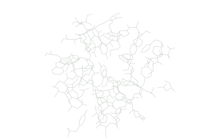
- >_ AgentInspect the receptor and public task requirements.1
- HarnessinputsExpose the task-bound molecular probe interface.1
All three points match. ✓
About this visualization
Drug-Design Agent Explorer. The visualization follows an agent as it works through three SMDD-Bench tasks: Lead Optimization, Scaffold Hopping, and Interaction Point Discovery. Each task exposes a different scientific workspace, from comparing closely related molecular edits, to balancing structural novelty against binding, to identifying recurring interaction hotspots inside a protein pocket.
Scientific Evidence. The agent builds its answer by combining deterministic chemistry checks with more expensive scientific measurements. Lead Optimization accumulates property and binding evidence across candidate molecules; Scaffold Hopping asks whether a structurally different molecule can preserve the reference binding interactions; Interaction Point Discovery reasons over spatial evidence inside a 3D binding pocket. What the model can infer depends on what information the harness makes visible and how that evidence is represented.
How to use it. Switch between tasks and move through the event ribbon to watch evidence accumulate over an agent run. Molecular structures, measurements, pocket geometry, and the working trace update together as the agent proposes candidates, calls tools, compares results, and submits an answer. Use Play to follow the sequence automatically, or pause to explore individual steps. The three views show how the same basic agent loop encounters different scientific problems depending on the environment around it.
Designing that interface by hand can matter a lot. SWE-agent showed that redesigning the interface through which a model interacts with a computer can substantially improve software-engineering performance (Yang et al., 2024). More recently, LangChain improved a fixed GPT-5.2-codex agent from 52.8% to 66.5% on Terminal Bench 2.0 through harness changes alone (Trivedy, 2026). Anthropic has similarly shown that long-running coding agents become substantially more capable when the surrounding harness manages task decomposition, context handoffs, and evaluation across extended runs (Young, 2025; Rajasekaran, 2026). François Chollet has described these increasingly elaborate outer systems as neurosymbolic architectures, where symbolic software orchestrates the neural model, its tools, and its execution (Chollet, 2026).
But how far can this go? Coding agents increasingly reuse a familiar set of harness components, including file viewers, search, test runners, and context handoffs. Scientific-agent harnesses exist too, but they are often designed around a particular domain and its tools. Agent Rosetta builds a specialized harness for protein design (Teneggi et al., 2026), and RetroAgent builds one around a structured search tree for retrosynthesis planning (Zhu et al., 2026). Moving to a new scientific setting can therefore reopen basic design questions about which tools the agent should have, what state should persist, and what it should observe. It also raises the question of how much of that design still has to come from a human.
We study this in the Small Molecule Drug Design benchmark, SMDD-Bench (Han et al., 2026), a collection of challenging, multi-turn agentic tasks in small-molecule design. Generative chemistry is a useful test of these questions because evaluating a candidate can require specialized scientific models, and several tasks depend on reasoning over 3D molecular structure.11. Boltz-2, which we shorten to Boltz below, lets us estimate whether a molecule is likely to bind to a protein without running a physical experiment. It is much cheaper than traditional simulation methods, but its predictions are still imperfect and can vary across protein targets. The agent may receive atom-level coordinates, the location of a binding pocket, or the spatial position of part of a molecule. How that information is presented to the model is itself part of the harness. What the model knows about the scientific problem therefore depends heavily on what the harness computes, remembers, and chooses to show it.
We focus on three SMDD-Bench tasks that expose different kinds of harness dependence. We first engineer their harnesses by hand, then ask whether an automated optimizer can discover the same kinds of improvements.
Our Testbed: SMDD-Bench
SMDD-Bench contains 502 instances across five small-molecule design tasks. Each combines chemical and biological reasoning with specialized tools, and several also require reasoning over the 3D geometry of a protein binding pocket.
We focus on Interaction Point Discovery, Lead Optimization, and Scaffold Hopping. They sit at very different points on the current capability curve. Lead Optimization is comparatively tractable, with the best reported model solving 57.6% of tasks, while the best reported pass rates for Scaffold Hopping and Interaction Point Discovery are only 3.8% and 4.0%, respectively.22. These are the best reported pass rates in the original SMDD-Bench evaluation: GPT-5.4 for Lead Optimization, GPT-5.4 / Claude Sonnet 4.6 / DeepSeek V3.2 tied for Scaffold Hopping, and Gemini 3.1 Pro for Interaction Point Discovery. Our Lead Optimization experiments below use the 68-task Lite subset. This gives us one task where agents already succeed reasonably often and two where performance remains close to the floor. The three tasks also ask the agent to do very different kinds of scientific work.
Interaction Point Discovery
The goal of Interaction Point Discovery (IPD) is to identify conserved interaction hotspots inside a protein binding pocket: regions where different molecules repeatedly make the same kinds of interactions when binding to the protein. These hotspots can then guide the design and optimization of new molecules.
The task contains a deliberate information asymmetry. The agent receives a single protein receptor and the location of its binding pocket, but the hidden answer is derived from interactions recurring across many different bound ligands, the molecules that bind to the protein. The agent must predict three ligand-side interaction points, specifying both their 3D coordinates and their pharmacophore type (the kind of chemical interaction the ligand feature can make, such as a hydrogen-bond donor, acceptor, or hydrophobic interaction).
Given a protein receptor and binding pocket, predict three conserved ligand-side interaction points.
This means the task is not simply asking which interactions look chemically plausible in the visible receptor. It asks which of those possibilities are likely to recur across a diverse set of binders. A chemically plausible interaction may therefore still be the wrong answer. And because the agent gets only three predictions, each one has to identify both the right interaction type and approximately the right location in 3D space.
How well do current agents perform?
Not great. Across the models evaluated in the original SMDD-Bench, only Gemini 3.1 Pro solved a single IPD task, while every other model scored 0/25. Our additional Qwen 3.5 9B baseline also solved 0/25.
But the all-or-nothing task metric hides substantial partial progress. GPT-5.4, for example, recovered 17 of the 75 individual interaction points while solving no complete tasks. Gemini recovered fewer points overall, 14/75, but was the only model to get all three points right on the same task.
This gap between point-level recovery and full-task success suggests that the models are not simply failing everywhere. They can often identify part of the answer, but those partial successes rarely come together into a complete prediction. To understand what was preventing that, we inspected the failed trajectories directly.
What are the agents getting wrong?
The first problem is that the visible receptor does not directly reveal the quantity being evaluated. Agents often inspected the binding pocket, identified chemically reasonable interaction sites, and treated them as likely conserved hotspots. But conservation is an ensemble property. The benchmark asks which ligand-side interactions recur across many different binders, not simply which interactions are plausible in a single receptor structure. A site can therefore make perfect chemical sense and still be a poor prediction of the hidden target.
A second failure was more basic. Models sometimes represented the interaction on the wrong side. The evaluator expects ligand-side pharmacophore points in empty pocket space, yet many trajectories instead selected receptor atoms themselves. This can also reverse the required interaction type. A hydrogen-bond donor on the protein, for example, implies a nearby ligand acceptor, not another donor placed on the receptor atom. In one audited AChE trajectory, the agent did exactly that.
Human acetylcholinesterase (AChE)
aWhat the agent predicted
bWhat the task asks for
A receptor donor implies a nearby ligand acceptor, not a donor on the receptor atom itself.
A separate problem appeared during final selection. Some trajectories spent more than one of their three predictions on the same hidden hotspot. Because each hidden point can be matched only once, a second prediction covering that region cannot earn another match. The CDK2 example below shows why simply spacing predictions apart is not enough. Two predictions were 2.757 Å apart, yet both still fell within the same hidden hotspot. With only three guesses available, the model needs to cover three distinct spatial hypotheses and localize each one accurately.
aTwo guesses cover one hotspot
CDK2 · GPT-5.4 submission
P1 and P2 both reach H1.
Only one can score.
3 predictions, 1 recovered hotspot
Hover, tap, or focus a prediction or hotspot.
bThree guesses cover three hotspots
Idealized comparison
Each prediction reaches a different hotspot.
All three can score.
3 predictions, 3 recovered hotspots
Prediction spacing is not enough. The three guesses must cover different hotspots.
There was also a simpler interface problem. The original harness exposed the same generic drug-design tools across tasks, even though IPD ultimately requires only three 3D points in a strict CSV format.33. Each row must contain four comma-separated fields: the x, y, and z coordinates followed by the pharmacophore type. The evaluator reads only the first three valid rows. The agent still had to choose tools, construct solution.csv, format it correctly, and submit the file manually. Those extra steps occasionally caused failures that had nothing to do with the scientific prediction. In smdd_002_Q92769_0, for example, the model produced three intended points but separated the values with spaces rather than commas, so the evaluator could not parse the submission.
These failures sit at different levels. Inferring conservation from a single receptor is part of the scientific challenge. Predicting receptor atoms instead of ligand-side features, covering the same hotspot twice, or losing an otherwise valid answer to file formatting are not. That distinction gave us a natural place to start improving the harness.
Fixing the representation
The first set of failures gave us a clear place to start. We refer to the original SMDD-Bench interface as V1, and the redesigned task-specific interface below as V2. We made it explicit that the model had to predict ligand-side interaction points in the pocket, rather than receptor atoms themselves. We also removed the tools that were irrelevant to IPD44. The original harness exposed the same generic drug-design interface across tasks, including ADMET property prediction and file-based submission. Most of these tools were irrelevant to IPD and added execution choices unrelated to predicting three interaction points. and replaced manual CSV construction with a dedicated submission interface that accepts the three predicted points directly.
That removed some avoidable execution burden, but it did not solve the central problem we saw in the trajectories. Even when the model identified chemically sensible regions of the pocket, it still had little evidence for deciding which of those interactions would actually recur across different bound ligands.
So we changed what the agent could observe. Instead of asking it to infer conservation entirely from a single receptor structure, we gave it a way to run small computational experiments. The agent could design probe molecules, use Boltz to predict their bound poses, the predicted 3D position and orientation of each molecule inside the pocket, and inspect the ligand-side pharmacophore features produced by each probe. By comparing several probes, it could build a small computational ligand ensemble of its own and look for interaction regions that appeared repeatedly.
The harness still did not choose which probes to generate or which recurring features to trust. Its role was to expose evidence that was closer to what the task actually asks about, while leaving the scientific decisions to the model.
V2 solved 2/25 complete tasks, but that terminal score compresses a lot of partial progress into a single number. Each submitted point can fail in two different ways: it can be in the wrong part of the pocket, or it can land near the right region but predict the wrong ligand-side feature type. Separating those two errors lets us see what the new representation actually changed.
We therefore look at point recovery in two ways. A coordinate-only match asks only whether the prediction lands within 2.5 Å of a hidden interaction point, ignoring its pharmacophore label. A type-compatible match uses the full benchmark criterion: the prediction must be close enough and specify a compatible ligand-side feature such as Donor, Acceptor, or Hydrophobic.55. The benchmark also matches submitted and hidden points one-to-one, so the same hidden hotspot cannot receive credit for multiple predictions.
On the same 25 Qwen 3.5 9B tasks, coordinate-only recovery rises from 19/75 under V1 to 47/75 under V2, while fully type-compatible recovery rises from 10/75 to 30/75.
The larger change is therefore spatial. V2 makes Qwen much better at finding regions that actually contain hidden interaction points. The remaining gap between 47 coordinate matches and 30 fully correct matches tells us that locating the hotspot and identifying the correct ligand feature are still separate problems.
V2 produces a large spatial gain; feature typing accounts for much of the remaining gap.
Support counts distinct probe molecules with a compatible extracted ligand feature near the submitted point.
A feature repeated across probes is more informative than a feature from any single predicted pose.
Repeated evidence across probes identifies better hotspots
Why does the probe representation improve localization? One possibility is simply that Boltz gives Qwen candidate coordinates to copy from. If that were enough, a feature seen in a single predicted ligand should already be useful.
We do not see that pattern. At a 1.5 Å support radius, final predictions supported by only one probe match a hidden point on 3/16 cases, almost identical to predictions with no supporting probe (3/13).
The signal becomes much stronger when multiple different probes place the same kind of ligand feature in approximately the same region. Among final points supported by at least two probes, 24/46, or 52.2%, match a hidden interaction point.
We refer to this agreement across probes as spatial recurrence. The value of the probe interface is therefore not simply that Boltz generates another set of coordinates. It gives Qwen a way to ask which ligand-side features keep reappearing across several independently predicted molecules.
That makes the computational experiment resemble the hidden task more closely. The benchmark target is constructed from interactions recurring across an ensemble of real binders, while V2 lets Qwen construct a small, noisy predicted ligand ensemble of its own.
CYP3A4
aOne receptor: plausible site
bLigand ensemble: conserved hotspot
Two predicted poses agree locally; the experimental ensemble does not.
The CYP3A4 example shows the limit of that proxy. Two independently predicted poses supported the same accessible aromatic region, yet that region did not correspond to a conserved hotspot in the aligned experimental ligand ensemble.
The probes themselves were already chemically diverse, with a mean within-task Morgan similarity of 0.159, but neither probe count nor scaffold diversity predicted better task performance. The two fully solved tasks actually used fewer probes on average than the failed tasks. What mattered more was spatial convergence across those probes, not simply how many molecules were generated.
Boltz binding probability was also only a weak guide to which individual feature was correct.66. Across extracted features, the correlation between the parent probe’s binding probability and feature correctness was 0.106. Mean binding probability was 0.347 for feature hits and 0.316 for misses. A binding score can help identify a broadly plausible pose, but every feature in that pose shares the same score, so it cannot identify which individual ligand feature corresponds to a conserved hotspot.
Better localization exposes a different bottleneck
The error distribution shows what remains after localization improves. Wrong-region predictions fall from 46/75 under V1 to 16/75 under V2, but 21/75 V2 predictions land near a hidden hotspot with an incompatible feature type. The new evidence is getting Qwen into the right parts of the pocket much more often; choosing the correct ligand-side chemistry within those regions is now the larger residual error.
P14061 makes this failure concrete. Its three submitted points were supported by 4, 3, and 1 probes, and all three landed close to hidden interaction regions. But all three were assigned incompatible feature types, so the task still scored 0/3.
The probe ensemble had therefore found the right parts of the pocket without solving the full semantic problem.
This also makes the role of the other V2 changes clearer. The redesigned harness explicitly states the strict 2.5 Å matching threshold, explains that each hidden point can match at most one prediction, and replaces file-based submission with a structured interface. Those changes make execution more reliable, but they do not explain the main improvement: duplicate-region errors do not decrease, while wrong-region errors fall sharply.
The main effect of V2 is therefore to improve the evidence Qwen has for where conserved ligand interactions are likely to occur. Once those regions become easier to find, assigning the correct ligand-side feature type becomes the next bottleneck.
Lead Optimization
IPD showed how much performance can depend on the representation exposed by the harness. Lead Optimization (LO) presents a different kind of problem. Instead of predicting three points in a binding pocket, the agent searches through a sequence of related molecules, repeatedly proposing candidates, testing them, and deciding what to change next.
Each task begins with a protein-bound reference molecule. The agent must improve one or more target properties while keeping the rest within specified ranges. A successful molecule must also preserve binding, satisfy the chemical constraints, and remain sufficiently similar to the reference. We measure this last requirement using Tanimoto similarity, which compares molecular fingerprints and gives higher values to more structurally similar molecules.
Adenosine A2A receptor · one target property, several requirements
Starting molecule
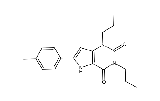
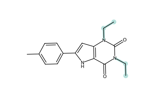
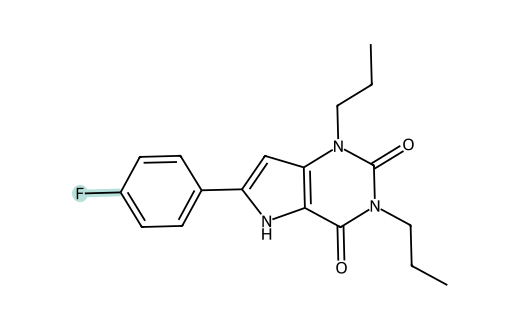
Reference before any chemical edit.
Task contract
Allowed region · hover or tap for details
Must improve
- Value
- 0.6862
- Required
- ≤ 0.5862
- Margin
- −0.1000
Outside requirement
Must stay in range
- Value
- 0.7627
- Required
- ≤ 0.8627
- Margin
- +0.1000
Pass
- Value
- 0.8375
- Required
- 0.7375 to 0.9375
- Margin
- +0.1000
Pass
- Value
- −5.7312
- Required
- ≥ −6.2312
- Margin
- +0.5000
Pass
- Value
- −0.7193
- Required
- ≤ −0.41927987039089204
- Margin
- +0.3000
Pass, reference baseline
Must still pass
- Value
- Not evaluated
- Required
- > 0.7000
- Margin
- —
Not evaluated
- Value
- 1.0000
- Required
- ≥ 0.7000
- Margin
- +0.3000
Pass
Hard chemistry constraintsAll pass
| Check | Required | Value |
|---|---|---|
| Sanitized SMILES | valid | valid |
| Molecular weight | < 600 | 325.412 |
| LogP | −1 to 5 | 3.28672 |
| TPSA | < 140 Ų | 59.79 |
| H-bond donors | ≤ 5 | 1 |
| H-bond acceptors | ≤ 10 | 2 |
| Rotatable bonds | ≤ 10 | 5 |
| Formal charge | −2 to +2 | 0 |
| SA score | < 4.5 | 2.321577 |
| PAINS | clean | clean |
| Brenk / NIH alerts | clean | clean |
Each track uses its own property scale.
Lead Optimization succeeds only when the target improves and every other requirement still passes.
The important part is that these requirements are coupled. An edit can fix the property being optimized while pushing something else out of range. In the example above, shortening both N-alkyl groups repairs CYP3A4 but causes binding affinity to fail. A different local edit, replacing the para-methyl group with fluorine, improves CYP3A4 while keeping the remaining requirements inside their allowed ranges.
The agent uses several tools to navigate these tradeoffs. RDKit performs deterministic checks such as molecular validity, structural constraints, and similarity. ADMET-AI predicts properties such as toxicity and permeability, while Boltz estimates whether a candidate is likely to preserve binding. Both ADMET and Boltz calls are limited, so the agent also has to decide which molecules are worth evaluating.
We refer to each requirement as a gate. A candidate succeeds only when every required gate passes.
How well do current agents perform?
Current models handle LO much better than IPD. On the 68-task Lite subset, GPT-5.4 and Gemini 3.1 Pro each solve 37/68 tasks, with Claude Sonnet 4.6 close behind at 36/68. This gives us something IPD did not: a substantial mix of successful and failed trajectories on the same task family.
Unlike IPD, Lead Optimization gives us enough successful and failed trajectories to study where capable agents diverge.
A terminal pass or fail, however, compresses a fairly long optimization process into a single bit. A candidate can satisfy the structural and property constraints but lose binding, preserve binding while missing one property target, or come very close to passing everything without ever becoming the submitted molecule. Looking at the evaluator stages gives us some indication of where these runs diverge. For example, GPT-5.4 and Gemini 3.1 Pro pass the Boltz binding stage on 89.7% of tasks, while Qwen 3.5 9B does so on 54.4%. Claude also performs strongly on the earlier checks but loses more candidates at the binding stage.
The search itself is long and state-heavy. A single trajectory can span dozens of turns while the agent proposes related analogs, evaluates different subsets of properties, discovers marginal constraint violations, tests binding, and later returns to candidates it considered much earlier. Across that process, it has to keep track of which measurements belong to which molecule, which requirements are still untested, which candidates remain viable, and how much evaluation budget remains.
Milestones C01 through C03 mark the key steps selected for this visualization, corresponding to positions C005, C009, and C033 in the model sequence of generated candidates.
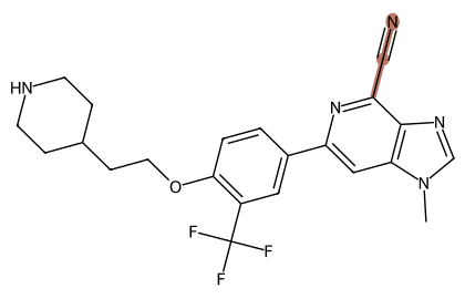
- BBB
- 0.8955pass
- Caco-2
- −5.0649pass
- CYP3A4
- 0.5322pass
- hERG
- 0.9739pass
- Binding
- > 0.70pass
- Similarity
- 1.0000pass
- Hard constraints
- 12 / 12pass
The starting molecule has a CN group (nitrile) which is commonly flagged in Ames assays.
Replace the nitrile while trying to preserve the properties the reference already satisfies.
Ames 0.6508 ×nitrile → dimethylamino
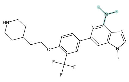 Ames is fixed, but binding is lost.
The starting molecule has a CN group (nitrile) which is commonly flagged in Ames assays.
Replace the nitrile while preserving the rest of the scaffold.
- Amestarget repaired
- 0.6508 → 0.5118✓ pass
- BBBwithin target range
- 0.9213✓ pass
- Binding probabilityrequired > 0.70
- 0.4656× fail
C005 fails binding probability (0.466 < 0.7). The Ames score is good … improve binding probability while maintaining Ames reduction.
Ames 0.6508 ×nitrile → hydroxymethyl
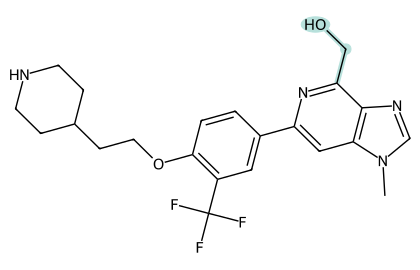 Binding is restored, but BBB becomes the next bottleneck.
I need to find modifications that won’t worsen binding too much but improve things marginally.
The model responds to C005’s binding failure with another nitrile replacement.
- Binding probabilityrequired > 0.70
- 0.8510✓ pass
- Amesrequired ≤ 0.5508
- 0.4425✓ pass
- BBBrequired ≥ 0.7955
- 0.7899× fail
missed by 0.0056
C009 has binding_probability = 0.8509 which is > 0.7! But bbb = 0.78985 which is below 0.7955 threshold.
Ames 0.6508 ×nitrile → hydroxyethyl
relative to C02: +CH₂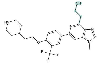 All gates pass.
The key insight: I need a molecule that combines good binding (like C009) with better BBB (like C005).
Add one methylene to C009’s hydroxymethyl group and reevaluate the narrow BBB miss.
- Amespass
- 0.4640✓ pass
- Binding probabilitypass
- 0.8492✓ pass
- BBBpass
- 0.8264✓ pass
Ames ✓ · Binding ✓ · BBB ✓ · Caco-2 ✓ · CYP3A4 ✓ · hERG ✓ · similarity ✓ · hard constraints ✓
C033 has passed all gates and is marked as “safe_to_submit”: true.
Reference baseline selected candidate · shaded regions satisfy the task requirement
Ames is fixed, but binding is lost.
In the original harness, the model had to track all of this information entirely within its own context. There was no centralized record linking each candidate to the measurements collected for it, the constraints it passed or failed, or the evaluations that were still missing. The trajectory above shows why this becomes difficult. A single molecular edit can repair one requirement while creating a new bottleneck, and the agent has to carry that updated state forward across many later turns.
Looking across the failed trajectories, this became a recurring pattern. The models could often propose reasonable candidates, but struggled to reliably keep track of what had already been tested, which evidence belonged to which molecule, and which candidate was actually the strongest by the end of the search. What initially looked like a molecular-design problem was therefore also a state-management problem.
What are the agents getting wrong?
Across the failed trajectories, the same general problem appeared at several different points in the search: the scientific state did not remain consistent over time.
A model could test a promising molecule, correctly discover that it failed a requirement, and then submit the same molecule later. When several related candidates were explored in parallel, measurements from one could be carried over to another, or an earlier candidate could disappear from consideration entirely. Even the task specification itself could drift. A one-sided constraint might later be remembered as a two-sided interval, changing which molecules the model considered viable.
The chemistry could remain useful while the state around it became inconsistent.
select a break to inspect the trajectory
The model changed the requirement while the search was running.
Kimi K2.5 · Cathepsin_K_20 · turns 23–24
The candidate satisfied the stated directional bound. It failed only after the task specification drifted inside the model’s working state.
- T00taskOriginal requirement
Keep solubility within 0.5 of the −4.8183 baseline, with a decrease tolerance. The operative lower bound was −5.3183.
- T22modelSearching for a better trade-off
“The thiomorpholine has very good Ames (0.503), good hERG (0.29), but clearance is 95.89—too high.” The model pivots to the methylpiperazine candidate.
- T22toolADMET · methylpiperazine_sulf
- clearance
- 66.7542
- Ames
- 0.5438
- hERG
- 0.3210
- BBB
- 0.5402
- solubility
- −3.8493
- T23modelFour passes, then a rejection
“This methylpiperazine_sulf candidate is very promising.” It marks clearance, Ames, hERG, and BBB as passes, then computes solubility as 0.969 from baseline and marks it ✗—because it has silently converted the directional tolerance into a symmetric interval.
- T24modelThe invented upper boundary becomes state
It writes the target as “−5.318 to −4.318,” calls −3.849 “too high,” and decides to add F, Cl, or other hydrophobic groups to lower solubility. The subsequent search is now optimizing against the model’s rewritten requirement.
The alias stayed fixed. The molecule underneath it did not.
Qwen 3.5 397B-A17B · CYP1B1_0 · turns 6–22
evidence attachedsimilarity 0.85
evidence attachedADMET · Boltz 0.875
Evidence from two molecular graphs was carried under one name. The contradiction appeared only when molecule B was rechecked exactly.
- T06modelCandidate family is defined
The model proposes converting aromatic methoxy groups to hydroxyls to lower LogP, increase solubility, and reduce BBB penetration. It assigns short aliases—including
c4—to the generated graphs. - T08modelThe first graph receives the label
“Candidates that have similarity ≥ 0.7: c1: Sim=0.74; c4: Sim=0.85.” At this point,
c4refers to the higher-similarity generated molecule. - T09toolDifferent graph, same alias
predict_admetis called on a hydroxyl-bearing graph recorded asc4. It returns hERG 0.4296, BBB 0.1452, solubility −4.4246, and CYP3A4 0.8269. Those results remain attached to the alias. - T15toolBinding evidence joins the mixed record
The second graph is passed to Boltz under
c4. It returns binding probability 0.874583 and affinity −1.137927, reinforcing confidence in the aliased candidate. - T22modelExact recomputation exposes the collision
“The similarity is 0.683, which is below 0.7 … c4 had similarity 0.85 but the canonical form showed 0.68.” The same name now carries the similarity of molecule A and the ADMET/Boltz evidence of molecule B.
One sample was treated as a distribution.
Claude Sonnet 4.6 · DHODH_12 · turn 8
Boltz budget after this call7 calls remained · nothing was sampled again
The observed margin was smaller than the variation between trajectory and evaluator calls, yet the single passing prediction was treated as certainty.
- T06modelA promising candidate is promoted
“mod5 (pyrazole CH₂OH) passes all ADMET constraints,” with solubility improved by about 1.07 and the remaining properties within tolerance. The model moves directly to a binding check.
- T08BoltzOne prediction lands just inside the gate
- affinity
- −1.652409
- required
- ≤ −1.637547
- margin
- 0.014862
- probability
- 0.932830
- calls left
- 7
- T09toolDeterministic checks all pass
MW 456.5, LogP 3.58, TPSA 98.4, Tanimoto 0.922, SA 3.10, and the PAINS/Brenk filters are verified. The report repeats the single Boltz value but does not test its stability.
- T10modelA sample becomes a fact
“All constraints are satisfied.” The checklist records affinity −1.652 with a difference of 0.285 ≤ 0.3 and binding probability 0.933, but contains no uncertainty estimate, repeat call, or acknowledgement that the margin is only 0.0149.
- T10writeSearch ends with budget unused
The model writes
solution.smi. Seven Boltz calls remain available; none are used to replicate the borderline result.
The agent wrote “fail,” then submitted the same molecule.
Kimi K2.5 · DHODH_14 · turns 46–48
- hERG
- 0.6648975
- required
- ≤ 0.663
FAIL (out by 0.002)
CCC[C@H](C)Oc1cc(…N(C)C…)ccc1CThis is visible in adjacent trace events: the failure was explicit, but the evidence did not survive into the final decision.
- T29ADMETThe disqualifying result first appears
- hERG
- 0.664898
- allowed
- 0.463–0.663
- BBB
- 0.477697
- CYP3A4
- 0.598056
- clearance
- 54.0797
- T30modelThe first comparison is internally inconsistent
It calls the candidate “very promising” and writes: “hERG: 0.665 … target range: 0.463–0.663 ✓ — within 0.102, just barely at edge.” The arithmetic exceeds both the upper bound and the stated ±0.1 tolerance, despite the checkmark.
- T31modelThe model notices the miss
“The hERG is slightly out of range (0.665 vs acceptable range 0.463–0.663). I need to reduce hERG slightly.” It proposes F, Cl, CF₃, and ester substitutions and continues searching.
- T37modelKnown failure becomes an accepted compromise
The model compares NMe2-meta—hERG out by 0.002—with F-meta—BBB out by 0.029—and decides “the NMe2 candidate is closer to target.” Closeness has silently replaced the requirement to pass every gate.
- T46verifyThe final ledger still contains two explicit failures
- hard constraints
- pass
- hERG
- 0.665 · fail
- Boltz probability
- 0.507 · fail
- reference probability
- 0.389
The verification says the result is “below 0.7” and that hERG is “out by 0.002.”
- T47modelThe same molecule is selected anyway
“Even though binding probability is below 0.7, this is the best candidate found.” It also notes “NMe2-meta: binding 0.507, ADMET known, hERG slightly off,” then writes that exact candidate to
solution.smi. - T48submitFile acceptance is not constraint success
The submission call again states hERG is 0.002 out of tolerance and binding probability is 0.507 versus the required 0.7. The harness responds only: “Submission accepted: solution.smi.”
The final edit created a molecule that had never been fully verified.
Claude Sonnet 4.6 · CDK2_20 · turns 32–35
CC(C)(C)c1cnc(…[C@H](O)[C@H](O)…)- Boltz
- ✓ measuredturn 32 · affinity −2.091
- Structural checks
- ✓ measuredturn 33 · all pass
- ADMET
- — missingbudget exhausted before this edit
- BBB
- — missinginferred from earlier analogs
A nearby molecule’s evidence was not evidence for the exact finalist. The last edit created a new candidate with empty ledger slots.
- T31modelTwo binding calls remain; ADMET is exhausted
The current 2Me-cyclohexanol candidate has 0.963 binding probability but misses the required affinity improvement. The model reasons that an extra hydroxyl could add a protein hydrogen bond while retaining Tanimoto similarity, then spends a remaining Boltz call on the 3,4-diol.
- T32BoltzThe new finalist wins on binding
- affinity
- −2.090998
- improvement
- 0.446397
- probability
- 0.975109
- calls left
- 1
The call rationale predicts that the added hydroxyl may interact with HIS82, HIS84, or ASP145.
- T33verifyOnly structural and binding evidence is complete
MW 383.5, LogP 3.41, TPSA 91.4, SA 4.00, Tanimoto 0.786, PAINS/Brenk, and Boltz all pass. The verification labels the remaining section: “ADMET (estimated, no ADMET budget left).”
- T34modelMissing measurements are replaced by directional guesses
“The key question is the ADMET constraints. Let me estimate based on what we know.” Lower LogP is used to infer improved solubility, lower CYP3A4, low hERG, and only a slight BBB decrease. No predictor is run on the exact finalist.
- T34writeThe inferred ledger is treated as complete
The exact 3,4-diol SMILES is validated syntactically and written to
solution.smi. The remaining Boltz call cannot answer the missing ADMET or BBB questions. - T35submitThe submission rationale repeats the inference
It claims the increased polarity “should also help maintain or improve ADMET properties like solubility and CYP3A4.” Official evaluation later measures BBB at 0.66895, below the required 0.6744.
The same issue showed up near the end of the search. A model might make a final structural edit and submit the new molecule without rechecking every requirement, or treat a single borderline Boltz result as stronger evidence than it really was. The chemistry could remain useful while the state surrounding it became inconsistent.
These failures have different surface forms, but they share the same underlying burden. In the original harness, candidate identity, task constraints, measurements, remaining evidence, and final verification all lived implicitly across the model’s context and tool outputs. As the trajectory grew longer, the model had to continually reconstruct the current state of the search for itself.
That suggested a different role for the harness. Rather than telling the model which molecules to design, we could move the parts of the search that are deterministic (candidate identity, constraint bookkeeping, evidence provenance, and submission checks) into the environment, while leaving molecular design and experimental choices to the model.
Fixing the state
The failures suggested a fairly simple division of responsibility. We still wanted the model to decide which molecules to make, which experiments were worth running, and how to respond to the results. But there was little reason for it to also reconstruct every threshold, remember which measurement belonged to which analog, or piece together the evidence for a finalist from dozens of earlier turns.
So we moved that state out of the trajectory and into the harness.
The task requirements were compiled once into an immutable specification with explicit thresholds and optimization goals.99. V2 does not expose hidden evaluator information. The optimization thresholds stored in the task specification are already given to the agent as part of the task, and the harness converts those public requirements into persistent, machine-readable state. This deliberately makes bookkeeping easier. Every unique molecule was assigned a persistent candidate ID, and its measurements were attached to that candidate in a central ledger. Deterministic checks such as molecular validity and constraint margins were computed by the harness, while ADMET and Boltz results were recorded directly against the exact molecule they evaluated.
The model still chose the chemistry. The harness made the facts durable.
The requirement is compiled once.
GPT-5.4 · ABL1_3 · V2 TaskSpec
solubility
- baseline
- −5.237
- comparator
- ≥
- threshold
- −5.737
- direction
- decrease
- tolerance
- 0.5
Reason over it. Do not rewrite it.The comparator and threshold are returned from the same stored object on every check.
This is an analogous V2 trajectory rather than a rerun of the exact Cathepsin_K_20 case in Fig. 13. It shows the mechanism that prevents a directional bound from becoming a reconstructed interval.
Related molecules receive distinct, durable identities.
GPT-5.4 · ABL1_11 · turn 17
OCc1ccc(F)cc1-c1ccc2cc(NC(=O)C3CC3)ncc2c1- parent
- C003
- similarity
- 0.7091
- ADMET
- attached to C007
- Boltz
- missing
CC(O)c1cc(F)ccc1-c1ccc2cc(NC(=O)C3CC3)ncc2c1- parent
- C003
- similarity
- 0.7455
- ADMET
- missing
- Boltz
- missing
same canonical graph as C003→rejectedCandidate C003 already has immutable parent C000.
The registry binds canonical structure, lineage, deterministic checks, and oracle outputs to one candidate ID. A new prose label cannot silently turn an existing graph into a different candidate.
Evidence arrives with the context needed to interpret it.
GPT-5.4 · Cathepsin_K_13 · turn 28
- observed
- −1.6753426
- comparator
- ≤
- threshold
- −1.6725892
- signed margin
- +0.0027533
- calls used
- 1
- calls remain
- 7
V2 does not remove stochasticity or decide whether one replicate is enough. It keeps the raw value, comparator, signed margin, replicate count, candidate identity, and remaining budget adjacent.
The model can inspect the live ledger instead of reconstructing it.
GPT-5.4 · BACE1_11 · turn 20 · V2.0.1
| candidate | evidence stage | failed gates | missing gates | limiting margin | relation |
|---|---|---|---|---|---|
| C003 | ADMET complete | BBB | Boltz probability | −0.028531 | frontier |
| C004 | ADMET complete | CYP3A4 | Boltz probability | −0.006714 | frontier |
| C009 | ADMET complete | CYP3A4 BBB | Boltz probability | −0.142795 | dominated by C003 |
C003 ↔ C004complementary near-passesC003 passes CYP3A4; C004 passes BBB.
C009within-set dominatedSame evidence stage; worse measured task gates than C003.
The view exposes failures, missing evaluations, lineage, signed margins, and dominance. It organizes evidence without recommending the next molecule or experiment.
Submission checks the exact candidate’s ledger.
GPT-5.4 · A2A_Adenosine_0 · turns 8–16
- BBB✕ 0.95089 outside [0.7375, 0.9375]
- Boltz affinity? missing
- Boltz probability? missing
ADMET 14 · Boltz 8 remain
Actionable evaluations still exist.
- failed gates✓ none
- missing gates✓ none
- verified file✓ exact contents
Binding probability 0.76461
Overall candidate state: pass.
Normal submission requires complete passing evidence for the registered candidate being submitted. A file-write success can no longer masquerade as scientific validity.
Long trajectories created a second problem. Even with the scientific state stored explicitly, the conversational history could become large enough that earlier reasoning and failed approaches were difficult to recover. Inspired by Agent Rosetta’s (Teneggi et al., 2026) approach to summarizing long scientific trajectories,1010. Agent Rosetta keeps a compact summary of earlier actions and their effects on design metrics, with only the two most recent steps kept verbatim. We borrow this split between long-term summary and recent context, but keep the candidate ledger outside the compressed conversation entirely. once the context grew beyond roughly 60K tokens, we asked the same model to compress the older trajectory into a summary of what had been tried, what had been learned, and what remained worth exploring. The most recent actions stayed verbatim, while the candidate ledger remained untouched.
We could thus compress the model’s memory of the search without compressing the scientific record itself. Older reasoning could be summarized, but candidate identities, measurements, failed constraints, and missing evidence remained exact.
Submission became stateful as well. Instead of asking the model to write an arbitrary molecule to solution.smi, the redesigned harness required it to submit a registered candidate directly. A normal submission was accepted only when that exact molecule had complete passing evidence. An incomplete or failed candidate could still be forced through as a fallback, but doing so became an explicit choice rather than an accidental mismatch between what had been measured and what was submitted.
The harness still did not choose which molecule to propose, which candidate deserved an expensive evaluation, or what chemical edit to try next. It made the facts of the search durable while leaving the molecular-design decisions to the model.
Did better state management help?
For Qwen 3.5 9B, the change was substantial. On the same 68-task Lead Optimization Lite subset, successful tasks increased from 13/68 to 33/68, raising the pass rate from 19.1% to 48.5%.
The redesigned harness also made the execution much cleaner. Under V1, the same molecule was sometimes sent to ADMET or Boltz multiple times even though an earlier result was already available. Across the 68 tasks, this produced 208 repeated ADMET calls and 24 repeated Boltz calls. Because V2 stored each result against the molecule’s canonical identity and reused it automatically, those counts fell to zero and two, respectively. V2 also stopped spending Boltz calls on molecules that had already failed deterministic structural checks.
The same difference appeared at submission time. Under V1, the model could submit a molecule even when an earlier measurement had already shown that it failed a required property, or when some required evidence had never been collected. V2 instead recomputed submission eligibility from the candidate’s stored evidence. A normal submission was accepted only when that exact molecule had complete passing measurements. Otherwise, the model had to continue searching or explicitly force a known-incomplete fallback.
13→33/ 68
tasks solved19.1% → 48.5%
66→48
terminal submissions97.1% → 70.6%
19.7%→68.8%
pass rate among submissions
one cell = one task · hover, tap, or focus a category
V1 records the final result; V2 also records why a submission was allowed or forced.
Turns
Tokens
ADMET calls
Boltz calls
More tasks were solved with fewer turns and tokens, even as the agent spent more of its budget on expensive structure checks.
These changes made the scientific state considerably more reliable, but they did not make the molecular search itself easy. V2 blocked 22 attempts to normally submit a failed or incompletely evaluated candidate. Nine of those trajectories continued searching afterward, but none subsequently found a passing molecule. The guardrail therefore prevented invalid submissions and made failures easier to interpret, but it did not itself manufacture successful chemistry.
The remaining failures make that distinction clearer. Among the 35 unsuccessful V2 trajectories, 22 ended exactly one measured requirement away from success, while most of the remainder were still blocked on multiple requirements. Binding affinity was the largest single bottleneck among the near-passes, accounting for 9 of those 22 tasks.
This is an important shift. Once candidate identity, measurements, and task state become reliable, the remaining question is increasingly how to discover or refine a molecule that satisfies the last difficult property, rather than how to remember which molecule passed which test.
The exact state representation would be more complicated in a real lead-optimization campaign. SMDD-Bench gives us explicit requirements, while real programs may involve noisy assays, changing priorities, conflicting measurements, or trade-offs that cannot be reduced to a fixed pass/fail gate. But the underlying separation still applies: candidate identity and experimental evidence can remain authoritative even when the policy for interpreting that evidence changes. A real system could therefore keep a stable scientific record while allowing the campaign objectives above it to evolve.
Lead Optimization produced a different dynamic than IPD. In IPD, the largest gain came from changing the evidence the model could observe. Here, much of the necessary evidence already existed, but keeping that evidence consistent across a long, multi-candidate search was itself a bottleneck. Externalizing that state did not solve the chemistry directly. It removed avoidable execution failures so that the remaining difficulty was increasingly the chemistry itself.
Scaffold Hopping
Scaffold Hopping asks the agent to do something almost opposite to Lead Optimization. Instead of staying close to the reference molecule, the new candidate must be structurally different enough to count as a new scaffold, the core molecular framework around which the rest of the molecule is built, while preserving the way the original molecule interacts with the protein pocket.
We refer to these two requirements as novelty and interaction preservation. In simple terms, novelty asks whether the molecule has changed enough to count as a genuinely different scaffold, while interaction preservation asks whether the new molecule still makes the same important contacts with the protein in roughly the same places.
Those two goals pull in opposite directions. Moving farther away in chemical space makes it easier to satisfy novelty, but also makes it easier to disrupt the interactions and geometry that supported binding in the first place.
What is allowed to change, and what has to stay the same?
Lead Optimization
A2A adenosine receptor · 5NM2
small structural moveCH₃→F
hERG · BBB · solubility · affinity held within range ✓
Scaffold Hopping
Protein P43235 · 3KWZ
large structural movenew core→same contact geometry
similar pocket-interaction pattern
stay near the reference → improve the property profile
different molecule family → same pocket behaviour
Lead Optimization therefore rewards controlled local change. Scaffold Hopping asks the agent to change the molecular scaffold while preserving pocket behaviour.
How well do current agents perform?
Almost not at all. Across the 52 Scaffold Hopping tasks, no evaluated model solves more than two. Claude Sonnet 4.6, DeepSeek V3.2, GPT-5.4, and our additional Qwen 3.5 9B baseline each solve 2/52, while the remaining models solve one task or none.
2 / 52· 3.8%
This is a sharp contrast with Lead Optimization, where current models solve a substantial fraction of the benchmark. Here, the best strict pass rate is only 3.8%.
The few successes are also not concentrated on the same handful of tasks. Across all eight models, nine different tasks are solved at least once, with different models occasionally finding different successful scaffold hops. So the benchmark does not appear to contain one tiny universally solvable subset surrounded by impossible cases. Instead, useful solutions seem possible in several places, but current agents reach them only rarely.
That leaves an important question open: are agents failing because they cannot generate viable scaffold changes, or because promising candidates are being lost somewhere later in the search?
What are the agents getting wrong?
The terminal scores make Scaffold Hopping look uniformly hopeless, but the individual evaluation checks reveal a much clearer pattern.
Generating a structurally distinct molecule is usually not the bottleneck. Models regularly clear the Tanimoto and scaffold-novelty thresholds, and several also propose candidates with high predicted binding probability.
A molecule can therefore have a high predicted binding probability without preserving the interaction pattern of the reference molecule. Binding asks whether the molecule is likely to bind at all; interaction preservation asks whether it binds in the same way.
The consistent failure is preserving the reference interaction pattern inside the pocket. No model clears this requirement on more than 3 of the 52 tasks. GPT-5.4 passes the binding-probability threshold on 46/52 tasks, yet preserves the required pocket interactions on only 3/52. Claude is even more revealing: it satisfies the scaffold-novelty requirements on all 52 tasks and clears binding on 48, but preserves the reference interaction pattern on just 2.
So the problem is not simply finding novel chemistry that can still bind. Agents can often do both of those things independently. The difficult part is finding a different scaffold that preserves the same interaction geometry in the pocket.
Exposing binding geometry to the agent
One problem was how the original harness presented Boltz results. The binding probability was returned directly to the model, while the structural evidence needed to inspect the predicted binding mode remained inside generated structure files. Once the agent found a sufficiently novel molecule with a high binding probability, it was much easier to answer whether it bound than whether it bound in the same way as the reference.
But those are different requirements. Verifying a scaffold hop meant comparing the reference complex with the candidate’s predicted poses and reasoning about whether the important protein–ligand interactions had been preserved. Under the original interface, the model had to locate the generated structure files and reconstruct that comparison for itself.
We redesigned the harness to make this evidence easier to access. As in Lead Optimization, proposed molecules were registered under persistent candidate IDs and passed through deterministic novelty checks before spending a Boltz call. The protein and pocket configuration were also bound directly to the task.
The larger change came after Boltz. Instead of returning a scalar binding score alongside a directory of generated structures, V2 attached the result directly to the candidate and surfaced the predicted pose files explicitly.1212. The difference is easiest to see in the raw tool outputs. V1 surfaced the scalar score directly but returned only a directory containing the predicted structures:binding_probability: 0.1583affinity_pred_value: 0.7236cif_dir: boltz_results/call_1/...The agent then had to locate the individual CIF files itself before inspecting the poses.V2 instead attached the result to a registered candidate and returned the pose files explicitly:candidate_id: C001binding_probability: 0.1665pose_files:model_0.cifmodel_1.cif...model_9.cif The agent could now move directly from asking whether a candidate appeared to bind to inspecting how it was predicted to bind.
The harness still did not calculate the scaffold-hopping interaction score or tell the model which contacts had to survive. Deciding whether a pose preserved the important interactions, how to modify a candidate when it did not, and whether another experiment was worth running remained part of the model’s scientific reasoning. Final submission was also tied to the same registered candidate state rather than an independently written molecule.
This gave us a cleaner test of the remaining problem: if the agent could directly inspect both structural novelty and predicted binding geometry, would that be enough to turn promising candidates into successful scaffold hops?
Did exposing the binding geometry help?
The redesigned harness made the Scaffold Hopping workflow much cleaner, but it did not improve terminal success.
Under the original harness, Qwen 3.5 9B reached submission on 39/52 tasks. V2 reached submission on 51/52 and produced valid evaluated candidates on 50. It also moved substantially more tasks through the earlier requirements: scaffold-novelty passes increased from 36 to 50, while candidates clearing the binding-probability threshold doubled from 14 to 28.
2 / 52→1 / 52
despite 51 / 52 runs reaching submissionV2 advances more tasks through submission, novelty, and binding before the interaction-preservation gate reverses the trend.
V2 reaches more submissions while using fewer resources
Total tokens
−40%Total turns
−22%Boltz calls
−10%51/52 trajectories reached submission, up from 39/52, despite using fewer tokens, turns, and Boltz calls overall.
The cleaner harness made the remaining bottleneck much easier to see, even if it could not solve it.
But those gains stopped at the interaction-preservation gate. Terminal success did not improve, moving from 2/52 under V1 to 1/52 under V2. The same pattern appears one step earlier: three V1 candidates preserved the required reference interaction pattern, compared with only one under V2.
The two harnesses did not simply recover the same easy cases either. V2 solved a new task, but lost both tasks solved under the original harness. So the cleaner interface changed which parts of the search succeeded without producing a reliable improvement in the final scientific objective.
This is very different from Lead Optimization. There, externalizing state removed enough avoidable failure to produce a large gain. Here, exposing the predicted poses made it easier for the model to inspect what had happened, but seeing the binding geometry was not the same as knowing how to preserve it. The model still had to decide which interactions mattered, which structural changes would retain them, and how to redesign the scaffold when they were lost.
The redesigned harness was also more efficient. It used roughly 40% fewer tokens and 22% fewer turns, while reaching substantially more submissions and using slightly fewer Boltz calls. So the lack of improvement was not simply the result of giving the model less opportunity to search.
At this point, the obvious next interventions start to move beyond representation and execution. We could explicitly extract the reference interactions, score how closely candidate poses reproduce them, or suggest structural edits that restore missing contacts. But each of those choices encodes more of the Scaffold Hopping strategy into the harness itself.
The asymmetry in V2 makes this boundary clear. The harness became very good at enforcing one side of the task (structural novelty) without becoming correspondingly better at preserving the reference interaction pattern. Looking at those two objectives separately helps explain why a cleaner and more reliable workflow still failed to improve terminal performance.
V2 solves novelty, not interaction preservation
Manual V2 makes novelty a hard prerequisite for structural evaluation. Every proposed molecule is first checked for both whole-molecule similarity and scaffold overlap against the reference, and a candidate cannot be sent to Boltz unless it passes both novelty gates.
This means V2 never spends its structural-evaluation budget on a molecule that is still too similar to the reference. Across all 236 Boltz-tested candidates, every molecule satisfied the benchmark’s novelty requirements.
The question is whether solving novelty actually helps with the harder objective: preserving the reference interaction pattern.
The molecules Qwen proposes under V2 suggest one reason for this asymmetry. Failed finalists contain, on average, only 73% as many heavy atoms as their reference molecules.1313. A molecule’s heavy-atom count is the number of non-hydrogen atoms in it. We use the candidate/reference ratio here as a coarse measure of molecular size: a ratio of 1.0 means the candidate has roughly the same number of non-hydrogen atoms as the reference, while 0.73 means it contains about 27% fewer. Across many trajectories, Qwen reaches a safely novel scaffold through fairly aggressive structural changes, often producing molecules substantially smaller than the reference.
That is effective for moving away from the reference in chemical space, but it gives the model little guidance on the competing objective: changing the scaffold while preserving the molecular architecture that supports the original interaction pattern. V2 verifies novelty, exposes the predicted poses, and keeps candidate evidence consistent, but Qwen still has to decide which anchors, substituents, linker lengths, and geometric relationships should survive the scaffold change.
The hard novelty gate may also make the search more conservative. Because candidates that fail novelty are blocked before Boltz, V2 cannot use them as intermediate structural experiments, even if their predicted poses might contain useful information for a later design. We do not see enough evidence to attribute V2’s poor interaction preservation to this restriction alone.
The practical bottleneck is therefore no longer enforcing novelty. It is proposing a molecule that is novel without changing so much of the reference architecture that the interaction pattern is lost.
What Was the Human Doing All This Time?
Looking back, the final interventions are easy to summarize. IPD needed ligand-side evidence. Lead Optimization needed durable candidate state. Scaffold Hopping made novelty and pose access reliable, but still left the molecular redesign strategy unresolved.
receptor-only view→ ligand-side probe evidence
implicit trajectory state→ authoritative candidate ledger
harness change
score-only feedback→ predicted poses
What took time was finding the right diagnosis.
The manual process was almost always the same: run agents, inspect failed trajectories, form a hypothesis about whether the failure came from the model or the harness, change the interface, rerun the benchmark, and inspect what broke next. Across the three task families, we went through hundreds of trajectories and repeated benchmark runs over roughly six weeks of iteration.
The difficult part was rarely implementing the eventual fix. It was deciding what kind of failure we were looking at.
In IPD, the model was trying to infer an ensemble-derived target from a single receptor. In Lead Optimization, a long multi-candidate search required the model to continually reconstruct candidate identity, measurements, and task status from its trajectory. In Scaffold Hopping, making novelty reliable and exposing predicted poses still left the model responsible for deciding what molecular architecture to preserve while changing the scaffold.
Those are very different diagnoses. None follows from a generic rule like “add more tools” or “write a better prompt.” The human contribution was deciding what the harness should represent explicitly, what it should make persistent, and what should remain part of the model’s scientific policy.
That boundary mattered because more harness engineering was not always better. Lead Optimization improved dramatically. IPD improved, then exposed a deeper probe-selection problem. Scaffold Hopping became cleaner and more efficient without improving terminal success. A harness change could remove accidental difficulty, or it could start encoding the scientific strategy itself.
Manual harness engineering was therefore far more than mere implementation work. It was an active search over representations, interfaces, and the boundaries between model and environment.
If harness engineering is itself a search process, how much of that search can we automate?
Can the Harness Engineer Itself?
There are already several ways to automate parts of harness design, including prompt optimizers such as GEPA (Agrawal et al., 2026). But our manual interventions changed much more than the prompt. Across the three tasks, we modified tools, state representation, context compaction, evaluators configured directly from each task, and submission logic. We therefore wanted to test automated harness engineering (AHE) in a setting where the entire executable harness could be part of the search space.
For this, we used Meta-Harness (Lee et al., 2026), which treats harness design itself as an iterative optimization problem.
The loop is straightforward. A meta-agent sees the harness implementations, execution traces, and evaluation scores from previous attempts, proposes a new executable harness, evaluates it with the same underlying agent model, stores the resulting code, traces, and score, and repeats.
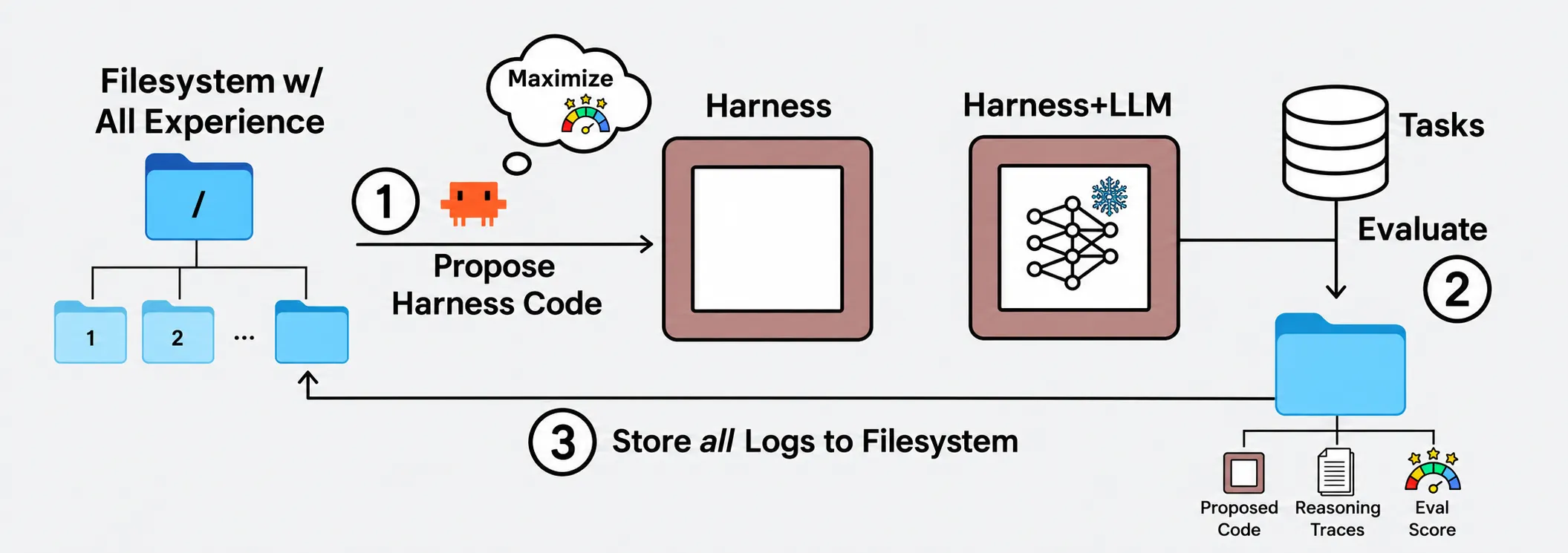
We initialized the search from the same original harness used at the start of our manual experiments. The question was whether automated search could recover the kinds of improvements we had spent weeks finding by hand.
We kept the same basic boundary around what counted as a valid harness intervention. The optimizer could reorganize public task information, change the tools and state exposed to the agent, and modify how the interaction loop was implemented. It could not expose hidden evaluator answers or directly insert known solutions into the environment. The downstream agent still had to produce a solution through interaction with the task.
There was another reason this comparison was useful. The manual phase was already partly model-assisted: Claude Opus 5 was used to help read trajectories, organize failure modes, and brainstorm possible harness changes. The human role was still to decide which hypotheses were worth pursuing, where the model–harness boundary should sit, and which interventions to implement.
AHE makes that division of labor much sharper. If a model can inspect the same traces, modify the harness itself, run the experiment, and use the resulting score to iterate, what is the human still contributing to the loop? Is the important part the search itself, or the judgment required to choose the right representation, abstraction, and boundary between harness and scientific policy?
How did we run the search?
To make the comparison clean, we kept the downstream scientific agent fixed. Qwen 3.5 9B solved the SMDD tasks in every run, while Claude Opus 5 acted as the meta-agent proposing changes to the harness around it. This isolates the object being optimized: the scientific agent stays the same, while the executable harness changes.
For each task family, AHE started from the same original harness used at the beginning of our manual experiments, rather than from the manually improved version. The meta-agent could inspect the current harness source code, trajectories produced by previous candidates, and their evaluation results, then propose a new executable harness for the next round.
We placed very few restrictions on what could change. Prompts were editable, but so were the tools themselves, the state exposed to the agent, tool outputs, context management, and the control logic around submission. In other words, the search space covered essentially the same parts of the system that we had spent the previous sections modifying by hand.
What stayed fixed was just as important. The child model, SMDD tasks, and underlying scientific evaluators did not change, and the optimizer received no hidden answers or known task-specific solutions. A candidate harness only earned reward by helping the same Qwen agent solve more tasks.
The same search protocol was run independently for Interaction Point Discovery, Lead Optimization, and Scaffold Hopping.
Who is optimizing whom?
redesigns the harness
solves the SMDD tasks
One harness evaluation
Every candidate harness is tested on the same search set.
Full search
base harness+10 new iterations
↓11 harness evaluations11×80=880
trajectories / task familyobjectiveterminal task success only
A candidate harness receives reward only when the child agent solves the complete task. No partial-credit signals, task-specific rubrics, or intermediate rewards are provided.
search spacefull executable harness
The meta-agent may modify prompts, tools, state representation, context handling, wrappers, control flow, and submission logic. The scientific agent, tasks, and evaluator remain fixed.
We ran the search independently for Interaction Point Discovery, Lead Optimization, and Scaffold Hopping. Each harness was evaluated on 20 tasks with four rollouts per task, giving 80 child-agent trajectories per harness. Starting from the base harness, Meta-Harness proposed 10 additional iterations, so each task family used 11 harness evaluations × 80 trajectories = 880 trajectories. Across the three searches, that produced 2,640 child-agent trajectories.
We deliberately kept the optimization signal simple: every harness was scored only by terminal task success, meaning whether the complete task passed all required checks. We did not add task-specific partial-credit rewards, failure-mode rubrics, or manually shaped intermediate objectives. That kept the comparison focused on the harness itself rather than giving the automated optimizer another layer of human-designed guidance through the reward.
This was a conservative choice for studying harness search, not necessarily the reward we would use if the only goal were to maximize benchmark performance.
Human Taste vs Automated Search
Automated harness engineering started from the same original harness and used the same raw materials as the manual process: code, trajectories, evaluation results, and repeated runs. The optimizer did not receive our diagnoses of what was wrong or which parts of the harness should change.
So did automated harness engineering recover the same improvements?
Not consistently. Manual V2 produced much larger gains on Lead Optimization and Interaction Point Discovery, while automated search found the strongest Scaffold Hopping harness.
Lead Optimization
Tasks solvedInteraction Point Discovery
Interaction points recoveredScaffold Hopping
Tasks solvedThe clearest endpoint gap was in Lead Optimization. The original harness solved 13/68 tasks, the selected AHE harness also solved 13/68, and Manual V2 reached 33/68. Automated search did discover much of the same high-level state-management problem: it added candidate registration, persistent notes, staged measurement, budget tracking, and finalist verification. The difference was how much of that state remained Qwen’s responsibility, and how much search the resulting system could reliably sustain.
Interaction Point Discovery showed the same pattern more clearly at the point level. The original harness recovered 10/75 hidden interaction points, automated search recovered 12/75, and Manual V2 recovered 30/75. Complete solutions remained rare, but the manual redesign produced a much broader shift in partial recovery rather than improving only a small number of tasks.
Scaffold Hopping was the exception. Automated search reached 5/52, compared with 2/52 under V1 and 1/52 under Manual V2. The absolute numbers remain small, so this is not evidence that Scaffold Hopping is solved. But it is the one task family where automated search found an intervention that moved terminal performance beyond both the starting harness and our manual redesign.
The interesting result is therefore not that one approach simply beats the other. Under this setup, the two search processes found different kinds of harness changes.
Our largest manual gains came when the main problem was the structure of the agent’s environment. In IPD, we changed what evidence the model could observe. In Lead Optimization, we made candidate state authoritative enough to support a much broader staged search. Automated search made only small gains on those tasks.
Scaffold Hopping was different. By the time we had cleaned up the representation and exposed the relevant geometry, the remaining problem was increasingly about how to search the chemistry itself. That was also the one setting where automated harness search did better than our manual redesign.
This split gave us a more useful question than “human or automated?”: what kinds of harness decisions are easy to discover through optimization, and which ones still depend on choosing the right representation of the problem in the first place?
The endpoint comparison tells us that manual and automated harness search produced different outcomes across the three tasks. It does not yet tell us what kinds of changes each process discovered. To understand that difference, we inspected the selected AHE harnesses and the trajectories they produced.
What Did the Automated Optimizer Actually Learn?
Lead Optimization
Automated search came closest here to the diagnosis we reached manually. The original harness left much of the search state inside Qwen’s trajectory, so Meta-Harness quickly began adding structure around candidate tracking, measurement, and submission.
Early iterations introduced a cheap-to-expensive workflow, persistent candidate notes, budget checkpoints, and explicit verification before submission. By iteration 2, candidates moved through more structured generation and measurement steps, objective completion was tracked explicitly, and the submitted molecule was checked against the candidate that had actually been evaluated. That iteration produced the highest observed reward and became the harness used in our final comparison.
The later search continued to elaborate the same basic idea. Automated optimization had therefore found much of the same high-level problem we had: a long Lead Optimization trajectory needs explicit machinery for keeping candidates, measurements, and requirements organized.
The primary distinction was where that state lived.
AHE gave Qwen a better procedure for maintaining the search state. It introduced candidate registration and persistent notes, but Qwen still had to combine raw ADMET outputs, local structural checks, task thresholds, candidate names, and current measurements into its own view of which molecules remained viable.
Manual V2 moved more of those joins into the environment itself. Candidate identity, task requirements, oracle results, missing measurements, and current gate status became authoritative program state rather than information the model had to repeatedly reconstruct from its context.
That difference still produced measurable execution failures under AHE. Across the 68 endpoint tasks, it repeated 89 ADMET evaluations and 8 Boltz evaluations on molecules it had already measured, and spent 20 Boltz calls on candidates that already failed deterministic structural checks. We also found 14 cases across nine tasks where the trajectory referred to one registered candidate while sending a different SMILES to the ADMET oracle. Manual V2 eliminated these classes of ambiguity by attaching evidence directly to canonical candidate identities.
But these execution errors do not explain the 20-success gap by themselves.
Both systems converted every fully passing molecule they discovered into a successful task. AHE found 13 such molecules, while Manual V2 found 33. The difference therefore appeared earlier, during candidate discovery and evaluation.
AHE 1.70%·Manual V2 1.50%
Similar per-candidate yield, a much wider search, and more complete solutions.
The performance gap therefore appears in how much search each harness can sustain, not in a large improvement in the quality of any individual proposal. Manual V2 carries many more candidates through the search while keeping their identities, measurements, and current status consistent.
The ledger makes that larger search easier to execute reliably. Known measurements can be reused, evidence stays attached to the correct molecule, and deterministic structural failures can be rejected before spending expensive evaluation budget. Its role is therefore not to preserve a single winning candidate until submission, but to keep a large multi-candidate search coherent as it expands.
Submission control played a different role. Manual V2 could block a failed or incompletely evaluated normal submission, but none of those blocked trajectories later became a success. The additional passing molecules were discovered during candidate generation and evaluation, not recovered at the final submission step.
AHE taught Qwen a better procedure for managing a Lead Optimization campaign. Manual V2 moved more of that campaign state into the environment and used it to support a substantially broader staged search. The result was not a dramatic increase in the quality of each individual proposal, but a search process that could explore and evaluate many more candidates without losing track of its own experiments.
Interaction Point Discovery
Automated search improved how Qwen reasoned about the receptor, but it did not change the source of evidence the model used.
Across iterations, AHE added increasingly structured geometric heuristics: mapping the cavity, identifying plausible receptor hotspots, scoring the three predictions jointly, controlling their spatial spread, and eventually distributing points through a ligand-sized pocket region.
Those changes helped localization. On the matched 25-task endpoint, coordinate-only recovery increases from 19/75 under V1 to 26/75 under AHE. But once the ligand-side feature type is included, the improvement is much smaller: 10/75 becomes 12/75.
Manual V2 behaves differently. It reaches 47/75 coordinate-only matches and 30/75 fully compatible matches. The gap is not simply that Manual V2 reasons more carefully about the same receptor. It gives Qwen a different source of evidence.
AHE never moved beyond using the receptor alone. Raw Boltz access existed in the runtime, but the selected harness explicitly framed IPD as a structure-geometry problem that did not require an oracle. Across the 25-task endpoint evaluation and every AHE search iteration, the agent made zero Boltz calls. One intermediate harness briefly introduced optional fragment probes, but none of its 80 trajectories used them, and the probe recipe disappeared again in the next iteration.
Manual V2 instead used Boltz on 24/25 tasks, producing 138 usable ligand poses and extracting 622 ligand-side pharmacophore features. Qwen could then compare those features across probes and prioritize regions where several predicted ligands independently placed compatible features.
As discussed earlier, this recurrence signal is substantially more informative than a single pose: at a 1.5 Å support radius, final points supported by at least two probes match 52.2% of the time, compared with 18.8% for points supported by only one probe.
The distinction is therefore not simply better versus worse geometric reasoning. AHE became better at asking where a ligand could plausibly interact with the visible receptor. Manual V2 gave Qwen evidence about where predicted ligands repeatedly placed interaction features. The latter is much closer to how the hidden target itself is constructed.
There is, however, another reason AHE underperformed: its reward hid most partial progress.
33 / 240 interaction points recovered
43 / 240 interaction points recovered
not visible to AHETerminal reward tracked partial progress poorly · r = 0.29
See how close each task got
20/20 ever reached ≥1 · 17/20 ever reached ≥2 · only 6/20 ever reached 3/3
The optimizer selected Harness 3 because it was the first harness to reach the maximum observed complete-task reward, with 2/80 successful trajectories and 33/240 matched points. A later harness recovered 43/240 points but solved only 1/80 complete tasks, so the terminal objective ranked it lower.
Selecting by point recovery would therefore have produced a stronger AHE harness for partial IPD performance. But it does not remove the representation gap. The better AHE harness still operates from receptor geometry, while Manual V2 introduces ligand-derived features and cross-probe recurrence.
The automated search was therefore improving a real subproblem, but mostly the wrong one. It became better at arranging plausible receptor-derived hypotheses, while Manual V2 changed the evidence from which those hypotheses were formed.
Scaffold Hopping
The selected AHE harness solved 5/52 tasks, compared with 2/52 under V1 and 1/52 under Manual V2.
The terminal numbers are still small, so we looked one level deeper at the two requirements that define a scaffold hop: changing the scaffold enough to be novel, while preserving the interaction pattern of the reference molecule.
Search and endpoint results are shown separately because they use different evaluation sets.
Across the search, stronger interaction preservation coincided with lower novelty reliability.
The automated harness preserved interactions more often, but passed the novelty gates less reliably.
The three harnesses fail very differently. Among evaluable submissions, V1 passes both novelty gates on 36/39 molecules and preserves the reference interactions on 3/39. Manual V2 pushes novelty to 50/50, but preserves the interactions on only 1/50. AHE moves in the opposite direction: only 29/45 evaluable submissions pass both novelty gates, while 8/45 preserve the required interaction pattern. AHE therefore does not make every part of the task more reliable. It improves interaction preservation while weakening novelty control.
AHE changes what Qwen proposes. The selected harness asks the model to preserve important anchors and substituents, maintain similar linker lengths and molecular size, and make relatively conservative changes to the central scaffold. Manual V2 verifies whether a molecule is novel and exposes the resulting Boltz poses, but leaves the choice of how to modify the scaffold to Qwen. AHE begins to encode that choice into the search procedure.
5 / 5
5 / 5
5 / 5
4 / 5
AHE mean1.06×
The successful molecules reflect that policy. Their heavy-atom counts range from 0.89× to 1.23× the reference, with a mean of 1.06×, while failed Manual V2 finalists average 0.73×. All five pass the authoritative novelty, interaction-preservation, and binding requirements, and four are the first successfully measured candidate in their trajectory. AHE is therefore producing full-sized, valid scaffold replacements without usually relying on a long repair sequence.
The improvement does not appear to come from a better interaction oracle or a stronger repair loop. AHE tells Qwen to inspect predicted contacts and compare them against the reference, but the harness does not calculate the benchmark’s interaction-preservation score or expose any equivalent scalar. Qwen still has to perform these comparisons itself through Python, and in practice those attempts are unreliable: we see failed pose parsers, missing paths, syntax errors, empty ligand selections, and incomplete contact comparisons. None of the five successes contains a trustworthy measured contact-overlap result that explains why the final molecule was selected.
The same trajectories show that AHE is usually not succeeding through a long propose–measure–repair loop. Four of the five successful tasks solve with the first molecule that receives a successful Boltz evaluation. Only 3KWZ_0 contains a substantial measured refinement sequence, and even there the useful feedback comes mainly from the binding score and chemical reasoning rather than a reliable measured comparison of the reference contacts. For most of the successful cases, the important difference appears before Boltz is called: AHE proposes a better candidate on its first serious attempt.
Novelty is also enforced less reliably under AHE. Manual V2 treats novelty as a hard, trusted gate: it uses the same novelty calculations as the benchmark evaluator, and a candidate cannot reach Boltz or normal submission unless it passes both the Tanimoto and scaffold-MCS thresholds.
AHE works differently. Instead of enforcing those checks inside the harness, it gives Qwen an RDKit recipe and asks the model to calculate novelty itself. That introduces two distinct failure modes.
First, the local calculation is not identical to the benchmark evaluator. In particular, AHE’s scaffold-MCS recipe uses different ring-matching settings, which can make a molecule appear more novel than it actually is.1414. The main mismatch is in the scaffold-MCS calculation. AHE uses ringMatchesRingOnly=True, which only allows atoms in a ring to match atoms in another ring when computing the maximum common substructure. The benchmark evaluator does not impose that restriction. This can make AHE report a smaller shared scaffold than the evaluator, making some candidates look more novel locally than they actually are under the benchmark. Manual V2 avoids this mismatch by calling the benchmark’s novelty functions directly. Replaying AHE’s local calculation on the endpoint candidates shows that 10 of the 45 evaluable finalists were classified as novel locally but failed the benchmark’s novelty check.
Second, the calculation is only advisory. Qwen can still submit a molecule even when its own local novelty check says the candidate should fail. This happens for another 6 of the 45 evaluable finalists.
Together, these two effects account for AHE’s 16 novelty failures at the endpoint: 10 false local passes and 6 cases where the local check itself indicated failure but the candidate was submitted anyway. Manual V2 avoids both problems by making novelty a deterministic harness-level gate rather than a model-managed procedure.
This weaker enforcement explains why AHE’s novelty pass rate falls to 29/45, but it does not explain away its successful scaffold hops: all five terminal successes pass the benchmark’s true novelty requirements.
Manual V2 and AHE also differ in what happens to a molecule that is not yet novel. V2 blocks that candidate before Boltz, while AHE can still evaluate it. In theory, that could matter: a molecule that cannot be submitted might still provide useful structural feedback before a later modification crosses the novelty threshold. We see little evidence that this mechanism explains AHE’s five successes. Four solve with their first successfully measured molecule, and only 3KWZ_0 goes through a longer measured sequence. The hard novelty gate may still remove useful exploratory candidates, but it does not appear to be the main observed difference between the two harnesses.
Taken together, the trajectories point to a simple contrast between the two harnesses. Manual V2 makes the constraints reliable: every molecule reaching Boltz is genuinely novel, evidence remains attached to the right candidate, and predicted poses are available for inspection. But the molecular redesign strategy remains Qwen’s responsibility. AHE makes that strategy more explicit: it tells Qwen which parts of the reference architecture to preserve and encourages conservative scaffold changes that remain close in size and geometry to the starting ligand.
The resulting harness has weaker novelty enforcement, but preserves the reference interaction pattern more often. The five successful trajectories also rule out several simpler explanations: all five are genuinely novel, four occur on the first successfully measured candidate, and none is explained by a reliable interaction-measurement loop. The strongest explanation supported by the current evidence is that AHE changed the distribution of molecules Qwen proposed, pushing the model toward minimally disruptive scaffold changes while Manual V2 focused on making novelty and execution exact.
Conclusion
So, is human taste overrated in harness engineering?
Not entirely. But these experiments suggest that its value depends heavily on what part of the system is being optimized.
The gains from harness engineering do carry over to scientific agents, but not uniformly. Automated search was quite capable of improving workflows inside an existing interface. It could add procedures, restructure tools, introduce memory, tighten submission logic, and even shape how the model searched the chemistry. But our largest manual gains came when the intervention changed the abstraction itself: what evidence the model could observe, what state the environment maintained for it, and what work the model should have to reconstruct at all.
The three tasks expose different versions of that boundary. Interaction Point Discovery improved when the harness stopped asking the model to infer conserved ligand behavior from a single receptor and instead exposed ligand-side features that could be compared for recurrence. Lead Optimization improved when candidate identity and experimental evidence became authoritative enough to support a much broader multi-candidate search. Scaffold Hopping marked the other side of the boundary: once novelty and execution were reliable, the remaining bottleneck was increasingly which chemistry to propose and which parts of the reference architecture to preserve.
This is consistent with scientific harnesses still being built around a particular task and its tools. Some parts of the interface can be standardized, but deciding what scientific information to represent explicitly, what the environment should enforce, and what should remain the model’s responsibility is itself part of the problem. That is where human judgment mattered most in our experiments. Once those choices are sensible, automated optimization may be able to search systematically over workflows, instructions, heuristics, and control policies without the same cycle of manual inspection and redesign.
It also gives us a practical stopping rule for manual harness engineering. Maintaining a deterministic state, exposing task-relevant evidence, and making execution reliable are natural jobs for the harness. As interventions begin to prescribe chemical transformations, prioritize particular interactions, or resolve scientific trade-offs, they increasingly become part of the model’s policy rather than infrastructure. At that point, improving the policy through training may be a cleaner lever than progressively hardcoding the strategy into the environment.
Human taste still matters in harness engineering. It is moving up a level, from fixing individual failures to deciding where the environment should end and the scientist should begin.
Once that boundary is chosen well, much of the optimization inside it may be automated.
Future considerations
SMDD-Bench has been useful precisely because its failures are difficult to classify cleanly as either “the model is bad at chemistry” or “the agent system is badly designed.” A model can propose useful chemistry and still fail because it loses track of evidence. A much cleaner harness can remove those failures and simply expose a harder scientific bottleneck underneath.
We have only explored part of that space. Interaction Point Discovery still has very sparse full-task success, Scaffold Hopping still struggles to preserve the reference interaction pattern, and the interventions here have not been evaluated across every model or SMDD-Bench task family. Tasks such as 2D Pharmacophore Identification and Fragment Assembly may put pressure on very different parts of the harness–policy boundary. The human-versus-automated patterns we saw here therefore need to be tested across more models, tasks, harnesses, and optimization procedures before treating them as general properties of scientific agents.
The optimization objective is another major open question. We intentionally gave AHE only terminal task success rather than task-specific partial-credit rewards. That kept the comparison cleaner, but Fig. 25 also shows what gets lost: in IPD, recovering zero, one, or two correct interaction points all looked identical to the optimizer unless the task was fully solved.
If the goal were purely to maximize performance, there are obvious alternatives. IPD could expose point-level recovery, Lead Optimization could use graded progress across evaluator gates, and other tasks could use evaluator-derived rubrics or richer intermediate rewards. The interesting question is whether better feedback simply makes automated harness search stronger, or whether it also changes what kinds of interventions it discovers.
There is also a natural next experiment on the model side. Once the harness has made the task legible, preserved the right state, and removed avoidable execution failures, does training the scientific policy produce larger and more transferable gains than continuing to engineer the environment around it?
Try it yourself
SMDD-Bench is available on Harbor and Prime as a runnable environment for launching trajectories, evaluating harnesses, and training agents against the benchmark.
Harbor: SMDD-Bench dataset
Prime: SMDD-Bench environment
We’re still improving these environments, so bug reports and contributions are very welcome.
Acknowledgments
We thank the broader SMDD-Bench team for building the benchmark and for discussions throughout this project. We’re also deeply grateful to Lambda for supporting the compute behind these experiments, to Anthropic (through its AI for Science program) and OpenAI for credit grants that made this work possible, and to the Foresight Institute, through its AI for Science & Safety Nodes program, for its compute support.
References
- Yang, J., Jimenez, C. E., Wettig, A., Lieret, K., Yao, S., Narasimhan, K., & Press, O. (2024). “SWE-agent: Agent-Computer Interfaces Enable Automated Software Engineering.” Advances in Neural Information Processing Systems (NeurIPS 2024).
- Trivedy, V. (2026). “Improving Deep Agents with Harness Engineering.” LangChain, February 17, 2026.
- Young, J. (2025). “Effective Harnesses for Long-Running Agents.” Anthropic Engineering, November 26, 2025.
- Rajasekaran, P. (2026). “Harness Design for Long-Running Application Development.” Anthropic Engineering, March 24, 2026.
- Chollet, F. (2026, August 6). Thread on agent harnesses as neurosymbolic architectures. X.
- Teneggi, J., Turzo, S. M. B. A., Marwah, T., Bietti, A., Renfrew, P. D., Mulligan, V. K., & Golkar, S. (2026). “Protein Design with Agent Rosetta: A Case Study for Specialized Scientific Agents.” arXiv preprint arXiv:2603.15952.
- Zhu, Y., Gan, J., Sun, X., Sun, F., Shi, Y., Islam, M. M., Shang, C., Gao, W., Coley, C. W., Sun, Y., & Wang, W. (2026). “RetroAgent: Harnessing LLMs to Search Over Structured Memory for Agentic Retrosynthesis Planning.” arXiv preprint arXiv:2607.14512.
- Han, K., Zhang, R., Wei, K., Mahdavi, H., Mireshghallah, N., & Barati Farimani, A. (2026). “SMDD-Bench: Can LLMs Solve Real-World Small Molecule Drug Design Tasks?” arXiv preprint arXiv:2605.21740.
- Agrawal, L. A., Tan, S., Soylu, D., Ziems, N., Khare, R., Opsahl-Ong, K., Singhvi, A., Shandilya, H., Ryan, M. J., Jiang, M., Potts, C., Sen, K., Dimakis, A. G., Stoica, I., Klein, D., Zaharia, M., & Khattab, O. (2026). “GEPA: Reflective Prompt Evolution Can Outperform Reinforcement Learning.” arXiv preprint arXiv:2507.19457.
- Lee, Y., Nair, R., Zhang, Q., Lee, K., Khattab, O., & Finn, C. (2026). “Meta-Harness: End-to-End Optimization of Model Harnesses.” arXiv preprint arXiv:2603.28052.
Citation
Please cite this work as:
Suresh Raghu, Kevin Han, Aviral Kumar, and Niloofar Mireshghallah.
"Is Human Taste Overrated in Harness Engineering,"
Suresh Raghu Blog, Oct 2, 2026.
And BibTeX:
@article{raghu2026humantaste,
  author  = {Suresh Raghu and Kevin Han and Aviral Kumar and Niloofar Mireshghallah},
  title   = {Is Human Taste Overrated in Harness Engineering},
  journal = {Suresh Raghu Blog},
  year    = {2026},
  month   = oct,
  day     = {2},
  note    = {https://r-suresh07.github.io/writing/is-human-taste-overrated-in-harness-engineering/}
}